Population

The population of the genetic algorithm is defined by an 2 dimensional array of individuals. Each individual is represented by a 1 dimensional array of genes. The number of genes in each individual is defined by the number of variables in the problem. The number of individuals in the population is defined by the population size. The population size is a parameter of the algorithm. The population size is the number of individuals in the population at any given time.

Population initialisation methods

Withing the genetic algorithm, the population is initialised using a population initialisation method. Included in the library are a number of methods that follow the same template.

All methods return a 2 dimensional array of individuals. Each individual is represented by a 1 dimensional array of genes. The number of genes in each individual is defined by the number of variables in the problem. A gene has a length of the bitsize of the variable.

Note

The binary to decimal conversion is done by the ndbit2int and int2ndbit methods these contain rounding errors for large bitsizes (>32) and small sizes (<4). For larger bitsizes the user should provide their own methods.

Random population initialisation

The random population initialisation method initialises the population with random values of 0s and 1s. This method is the most simple method of initialising the population and provides no information about the problem.

To compute an individual the following equation is used:

\[x = rand(0, 2)\]

Where \(x\) is the gene value and \(rand\) is a random number between 0 and 2.

These values are computed for the length of the individual. And stacked for the amount of individuals in the population resulting in the population matrix.

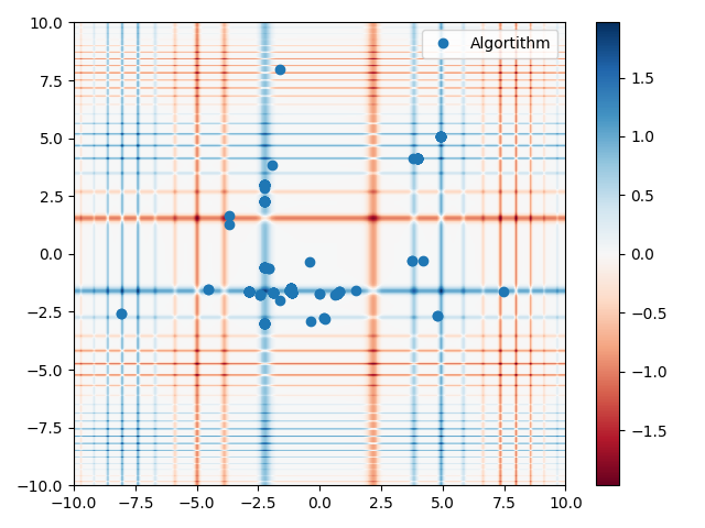
A two-dimensional representation of the population on the michealwicz function is shown below.

Random population initialisation on the michealwicz function.

Uniform population initialisation

The uniform population initialisation method initialises the population with uniformly distributed values between the lower and upper bounds of the variables. This method provides a boundary for values generated for the population. The floating point values can be bounded by using the factor and bias parameters.

Within the input space the following probability density function is defined to find values for the population:

\[\begin{split}f(x) = \begin{array}{lcl} \frac{1}{b - a} & \text{for} & a \leq x \leq b \\ 0 & \text{for} & x < a \text{ or } x > b \end{array}\end{split}\]

Where \(f(x)\) is the probability density function, \(b\) is the upper bound, \(a\) is the lower bound and \(x\) is the value of the gene.

To compute an individual the following equation is used:

\[x = rand(a, b)\]

Where \(x\) is the gene value and \(rand\) is a random number between the lower and upper bounds. These values are stacked into a matrix for the amount of individuals in the population and converted to binary using the int2ndbit() method with the factor and bias parameters.

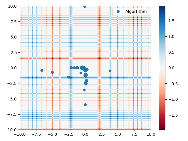
The figure below shows a two-dimensional representation of the population on the michealwicz function.

Uniform population initialisation on the michealwicz function.

Gaussian population initialisation

The gaussian population initialisation method initialises the population with normally distributed values with a location parameter of the mean and a scale parameter of the standard deviation. This method provides a boundary for values generated for the population. The floating point values can be bounded by using the factor and bias parameters.

Within the input space the following probability density function is defined to find values for the population:

\[f(x) = \frac{1}{\sigma \sqrt{2 \pi}} e^{-\frac{(x - \mu)^2}{2 \sigma^2}}\]

Where \(f(x)\) is the probability density function, \(\sigma\) is the standard deviation, \(\mu\) is the mean and \(x\) is the value of the gene.

To retain the normal distribution on the population the normally distributed values are “split” into m parts (the amount of individuals in the population) and then stacked into a matrix. This process is visualised in the figure below.

The cutting of the normal distribution into m parts for the population.

Each part consists out of n genes (the amount of variables in the problem). The matrix is then converted to binary using the int2ndbit() method with the factor and bias parameters.

The figure below shows a two-dimensional representation of the population on the michealwicz function.

Gaussian population initialisation on the michealwicz function.

Cauchy population initialisation

The cauchy population initialisation method initialises the population with cauchy distributed values with a location parameter of the mean and a scale parameter of the standard deviation. This method provides a boundary for values generated for the population. The floating point values can be bounded by using the factor and bias parameters.

Within the input space the following probability density function is defined to find values for the population:

\[f(x) = \frac{1}{\pi \gamma \left[ 1 + \left( \frac{x - \mu}{\gamma} \right)^2 \right]}\]

Where \(f(x)\) is the probability density function, \(\gamma\) is the scale parameter, \(\mu\) is the location parameter and \(x\) is the value of the gene.

The population is generated in the same way as the gaussian population to retain the cauchy distribution. The figure below shows a two-dimensional representation of the population on the michealwicz function.

Cauchy population initialisation on the michealwicz function.

Differences between Python and C methods

The main difference between the Python and C methods is the addition of the :function:`normal_bit_pop_boxmuller` method. This method is used to generate normally distributed values for the population using the Box-Muller method.

This method can be generalised in the following two equations:

\[\begin{split}z_0 = \sqrt{-2 \ln{U_1}} \cos{(2 \pi U_2)} \\ z_1 = \sqrt{-2 \ln{U_1}} \sin{(2 \pi U_2)}\end{split}\]

Where \(z_0\) and \(z_1\) are the normally distributed values, \(U_1\) and \(U_2\) are uniformly distributed values between 0 and 1.

The other function uses the gaussian pdf in a similar fashion to the python method.

Python methods for population initialisation

Below are the library provided population initialisation methods. These methods are used to initialise the population of the genetic algorithm.

dfmcontrol.Utility.pop.bitpop(shape: list, bitsize: int = 8, factor=1.0, bias=0.0)

Generate a bit population within boundaries imposed by the factor, bias and bitsize. Using floats converted with int2ndbit and ndbit2int.

Parameters

• shape – Population size dtype tuple [individuals, variables]

• bitsize – Bitsize dtype int

• factor – Factor dtype float

• bias – Bias dtype float

Returns

List of random bits with a bit being a ndarray array of 0 and 1.

dfmcontrol.Utility.pop.cauchy_bit_pop(shape: Iterable, bitsize: int, loc: float, scale: float, factor: float = 1.0, bias: float = 0.0) → numpy.ndarray

Generate a cauchy bit population with floats converted with int2ndbit and ndbit2int.

Parameters

• shape – Population size dtype tuple [individuals, variables]

• bitsize – Bitsize dtype int

• loc – loc dtype float

• scale – scale dtype float

Returns

List of random bits with a bit being a ndarray array of 0 and 1.

dfmcontrol.Utility.pop.cauchyrand_bit_pop_IEEE(shape: Union[Iterable, float], bitsize: int, loc: float, scale: float) → numpy.ndarray

Generate a cauchy distributed bit population with floats converted with float2NdbitIEEE754 and NdbittofloatIEEE754.

Parameters

• shape – Population size dtype tuple [individuals, variables]

• bitsize – Bitsize dtype int

• loc – loc dtype float

• scale – scale dtype float

Returns

List of bits that are cauchy distributed with a bit being a ndarray array of 0 and 1.

dfmcontrol.Utility.pop.normal_bit_pop(shape: Iterable, bitsize: int, loc: float, scale: float, factor: float = 1.0, bias: float = 0.0) → numpy.ndarray

Generate a normal bit population with floats converted with int2ndbit and ndbit2int.

Parameters

• shape – Population size dtype tuple [individuals, variables]

• bitsize – Bitsize dtype int

• loc – loc dtype float

• scale – scale dtype float

Returns

List of random bits with a bit being a ndarray array of 0 and 1.

dfmcontrol.Utility.pop.normalrand_bit_pop_IEEE(shape, bitsize, loc, scale)

Generate a normal distributed bit population with floats converted with float2NdbitIEEE754 and NdbittofloatIEEE754.

Parameters

• shape – Population size (Individuals, genes) dtype tuple individuals

• bitsize – Bitsize dtype int

• loc – midpoint of the distribution

• scale – multiplier over the distribution

Returns

List of random bits with a bit being a ndarray array of 0 and 1.

dfmcontrol.Utility.pop.rand_bit_pop(n: int, m: int) → numpy.ndarray

Generate a random bit population, n individuals with m variables.

Parameters

• n – Population size dtype int

• m – Bitsize dtype int

Returns

List of random bits with a bit being a ndarray array of 0 and 1.

dfmcontrol.Utility.pop.uniform_bit_pop(shape: Iterable, bitsize: int, boundaries: list, factor: float = 1.0, bias: float = 0.0) → numpy.ndarray

Generate a uniform bit population with floats converted with int2ndbit and ndbit2int.

Parameters

• shape – Population size dtype tuple [individuals, variables]

• bitsize – Bitsize dtype int

• boundaries – Boundaries [0] lower, [1] upper dtype list of float or int

Returns

List of random bits with a bit being a ndarray array of 0 and 1.

dfmcontrol.Utility.pop.uniform_bit_pop_IEEE(shape: Union[Iterable, float], bitsize: int, boundaries: List[int]) → numpy.ndarray

Generate a uniform distributed bit population with floats converted with float2NdbitIEEE754 and NdbittofloatIEEE754.

Parameters

• shape – Population size dtype tuple [individuals, variables]

• bitsize – Bitsize dtype int

• boundaries – Boundaries dtype list [lower, upper]

Returns

List of random bits with a bit being a ndarray array of 0 and 1.

C methods for population initialisation

void bitpop(int bitsize, int genes, int individuals, int **result)

Fill a matrix with random bits.

Parameters

• bitsize (int) – The size of the integer in binary.

• genes (int) – The number of genes in an individual.

• individuals (int) – The number of individuals in the population.

• result (int**) – The matrix to be filled with random bits. shape = (individuals, genes * bitsize)

void uniform_bit_pop(int bitsize, int genes, int individuals, float factor, float bias, int normalised, int **result)

Fill a matrix with bits according to a uniform distribution.

Parameters

• bitsize (int) – The size of the bitstring.

• genes (int) – The number of genes in the bitstring.

• individuals (int) – The number of individuals in the bitstring.

• factor (float) – The factor by which the uniform distribution is scaled.

• bias (float) – The bias of the uniform distribution.

The factor and bias are used to calculate the upper and lower bounds of the uniform distribution according to the following formula: [1]

\[\begin{split}upper = round((bias + factor) * 2^{bitsize}) \\ lower = round((bias - factor) * 2^{bitsize})\end{split}\]

Which results in the integer domain between round(lower * 2^{bitsize}) and round(upper * 2^{bitsize}).

Parameters

• normalised (int) – Whether the uniform distribution is normalised.

• result (int**) – The matrix to be filled with bits according to a uniform distribution. shape = (individuals, genes * bitsize)

References

1

https://stackoverflow.com/questions/11641629/generating-a-uniform-distribution-of-integers-in-c Lior Kogan (2012)

void normal_bit_pop_boxmuller(int bitsize, int genes, int individuals, float factor, float bias, int normalised, float loc, float scale, int **result)

Fill a matrix with bits according to a normal distribution. using the following probability density function:

\[f(x) = \frac{1}{\sigma \sqrt{2 \pi}} e^{-\frac{1}{2} (\frac{x - \mu}{\sigma})^2}\]

Calculate them using a Box-Muller transform, where two random numbers are generated according to a uniform distribution and then transformed to a normal distribution with the following formula: [1]

\[\begin{split}z_0 = \sqrt{-2 \ln U_1 } \cos{(2 \pi U_2)} \\ z_1 = \sqrt{-2 \ln U_1 } \sin{(2 \pi U_2)}\end{split}\]

Where \(U_1\) and \(U_2\) are random numbers between 0 and 1.

Parameters

• bitsize (int) – The size of the bitstring.

• genes (int) – The number of genes in the bitstring.

• individuals (int) – The number of individuals in the bitstring.

• factor (float) – The factor by which the normal distribution is scaled.

• bias (float) – The bias of the normal distribution.

The factor and bias are used for the conversion to the integer domain according to the following formula:

\[float = (int - bias) / factor\]

Parameters

• normalised (int) – Whether the normal distribution is normalised.

• loc (float) – The mean of the normal distribution.

• scale (float) – The standard deviation of the normal distribution.

• result (int**) – The matrix to be filled with bits according to a normal distribution. shape = (individuals, genes * bitsize)

References

1

https://en.wikipedia.org/wiki/Box%E2%80%93Muller_transform Wikipedia contributors (2019)

void normal_bit_pop(int bitsize, int genes, int individuals, float factor, float bias, int normalised, float loc, float scale, int **result)

Produce a normal distributed set of values using the Gaussian distribution:

\[f(x) = \frac{1}{\sigma \sqrt{2 \pi}} e^{-\frac{1}{2} (\frac{x - \mu}{\sigma})^2}\]

Where x is linearly spaced between (-factor and factor) + bias.

Parameters

• bitsize (int) – The size of the bitstring.

• genes (int) – The number of genes in the bitstring.

• individuals (int) – The number of individuals in the bitstring.

• factor (float) – The factor by which the normal distribution is scaled.

• bias (float) – The bias of the normal distribution.

The factor and bias are used for the conversion to the integer domain according to the following formula:

\[float = (int - bias) / factor\]

Parameters

• normalised (int) – Whether the normal distribution is normalised.

• loc (float) – The mean of the normal distribution.

• scale (float) – The standard deviation of the normal distribution. Due to the use of floats the scale should be > 2.

• result – The matrix to be filled with bits according to a normal distribution. shape = (individuals, genes * bitsize)

void cauchy_bit_pop(int bitsize, int genes, int individuals, float factor, float bias, int normalised, float loc, float scale, int **result)

Produce a normal distributed set of values using the Cauchy distribution:

\[f(x) = \frac{1}{\pi \gamma [1 + (\frac{x - x_0}{\gamma})^2]}\]

Where x is linearly spaced between (-factor and factor) + bias.

Parameters

• bitsize (int) – The size of the bitstring.

• genes (int) – The number of genes in the bitstring.

• individuals (int) – The number of individuals in the bitstring.

• factor (float) – The factor by which the normal distribution is scaled.

• bias (float) – The bias of the normal distribution.

• normalised (int) – Whether the normal distribution is normalised.

• loc (float) – The location of the peak of the distribution.

• scale (float) – The width of the distribution.

• result (int**) – The matrix to be filled with bits according to a normal distribution. shape = (individuals, genes * bitsize)